마이닝에서 알다싶이 무언가를 캐낸다라는 맥락이다. 즉 테스트 마이닝은 텍스트(텍스트 데이터)에서 무언가를, 인사이트를 캐낸다라는 뜻
텍스트 데이터는 비정형인데 텍스트 마이닝에서 가장 중요한 부분은 비정형 데이터를 사용 가능하도록 정형 데이터로 바꿔주는 작업이다
워드클라우드 시각화, 감성분류 등이 텍스트 마이닝을 혼합한 기법으로 볼 수 있다
02 텍스트를 계산 가능한 데이터로 처리하는 방법
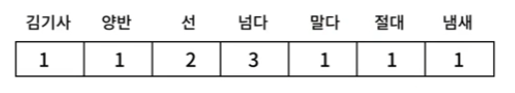
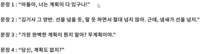
BoW(Bag of Words) - 형태소를 추출하는 방법 "김기사 그 양반. 선을 넘을 듯, 말 듯 하면서 절대 넘지 않아. 근데, 냄새가 선을 넘지." 라는 문장에서 불용어가 아닌 형태소를 추출 → ['김기사','양반','선','넘다','말다','절대','냄새'] 이렇게 형태와 의미를 가진 단어를 추출 →추출한 단어가 몇번 등장하는지 카운팅 [1,1,2,3,1,1,1] → 최종적으로 벡터 형태로 만듬 원핫인코딩이랑 비슷하지만 각 단어가 얼마나 등장했는지에따라 벡터형태로 넣어 준다
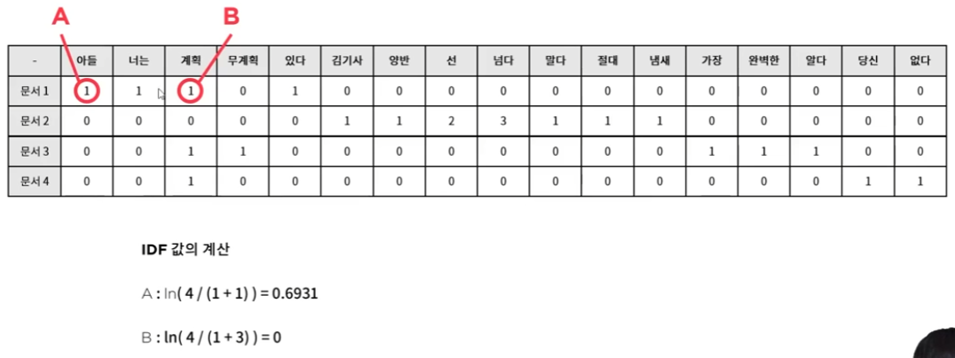
문서 단어 행렬(Document-Term Matrix, DTM) - 데이터가 여러 문장이 되었을 때 사용 여기서 모든 단어들을 형태소 기반으로 추출함
단어의 중요도를 계산하는 방법 (Term Frequency-Inverse Document Frequency, TF-IDF) 위의 방법들로는 단순 단어들이 얼마나 등장했는지 카운터를 하는 용도이다. 그래서 이 카운터만 보고는 어떤 단어가 중요한지 구별 하기 힘들다. 이때 쓰는 방법이 'TF-IDF'
쉽게 말해 TF-IDF는 이 특정 문장에서는 많이 등장했지만 다른 문장에서는 등장 하지 않았으니 그 단어가 이 문장에서 중요한 단어이다 라고 계산을 하여 내놓는다. 여기서 보면 계획은 0으로 너무 많이 등장해서 단어의 중요성이 떨어지고, 아들은 0.7에 가깝기때문에 중요하다고 볼 수 있다
03 텍스트 데이터 전처리
BoW를 통해 텍스트 데이터를 벡터단위로 변경하고 TF-IDF를 통해 중요도를 체크 할 예정
* 기본 필수 라이브러리
import pandas as pd
import numpy as np
import matplotlib.pylab as plt
import seaborn as sns

import warnings
warnings.filterwarnings('ignore')

df = pd.read_csv("https://raw.githubusercontent.com/yoonkt200/FastCampusDataset/master/bourne_scenario.csv")

df.head()
※구글에서 무비스크립트를 치면 무료로 영화 시나리오들을 받을 수 있다. 좋은점은 스크립트가 일정한 규칙으로 나열되 있다.
처리 하기 좋도록 스크립트가 규칙에 의해 나열되어있다.
항상 EDA부터 진행 해야 한다!
# 데이터 개수
df.shape
(320, 3)
# 널값 확인
df.isnull().sum()
page_no 0
scene_title 0
text 0
dtype: int64
# 데이터 형태 확인
df.info()
# Column Non-Null Count Dtype
--- ------ -------------- -----
0 page_no 320 non-null int64
1 scene_title 320 non-null object
2 text 320 non-null object
# 실제 사용하고자 하는 데이터 형태 확인
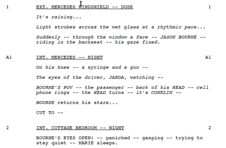
df['text'][0]
" 1 It's raining... Light strobes across the wet glass at a rhythmic pace... Suddenly -- through the window a face -- JASON BOURNE -- riding in the backseat -- his gaze fixed. "
사용하고자 하는 'text' 데이터에 전처리가 많이 필요해 보인다. 공백, 특수 문자 등 처리를 해줘야 한다.
정규 표현식을 사용하여 텍스트 데이터 전처리
# 정규식을 써 숫자, 공백, 특수문자, 대문자, 를 제거해 통일을 해야 한다.
import re

def apply_regular_expression(text):
    text = text.lower()
    english = re.compile('[^ a-z]') # '^' = 모두 들고 옴, 즉 '^ _____' 으로 띄어쓰기+a-z만 들고옴(나머지 특수문자 없어짐)
    result = english.sub('', text) #.sub() - 정규표현식을 들어오는 text파라미터에 적용함
    result = re.sub(' +', ' ', result) # ' +' = 띄어쓰기가 2개이상이면 ' ' 하나로 바꿔 줘
    return result

apply_regular_expression(df['text'][0])
' its raining light strobes across the wet glass at a rhythmic pace suddenly through the window a face jason bourne riding in the backseat his gaze fixed '
" 1 It's raining... Light strobes across the wet glass at a rhythmic pace... Suddenly -- through the window a face -- JASON BOURNE -- riding in the backseat -- his gaze fixed. "
text = a.lower() text
" 1 it's raining... light strobes across the wet glass at a rhythmic pace... suddenly -- through the window a face -- jason bourne -- riding in the backseat -- his gaze fixed. "
result = english.sub('', text) result
' its raining light strobes across the wet glass at a rhythmic pace suddenly through the window a face jason bourne riding in the backseat his gaze fixed '
result = english.sub('!', text) result
' ! it!s raining!!! light strobes across the wet glass at a rhythmic pace!!! suddenly !! through the window a face !! jason bourne !! riding in the backseat !! his gaze fixed!
전처리 한 데이터를 다시 붙여 주자
# 컬럼을 새로 만들어 적용된 전처리 텍스트를 붙여주자
# df['preprocessed_text'] = df['text'].apply(apply_regular_expression)
df['preprocessed_text'] = df['text'].apply(lambda x: apply_regular_expression(x))
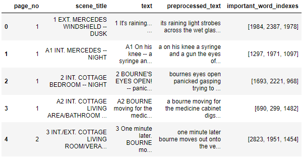
df.head()
※ 람다 함수를 잘 기억해야한다. .apply() 함수는 열 혹은 행에 대해 함수를 적용하게 해주는 메서드이고 def(x): 로 선언된 함수의 return값을 모든 데이터 프레임에 적용할때 apply()를 쓴다. 그리고 lambda 함수는 .apply()를 더 쉽고 빠르게 각 행과 열에 적용 시켜줌. 따로 공부 할 필요가 있음
BoW 적용
- 이제 전처리 된 텍스트들을 말 뭉치로 바꾸고 그 각각의 말뭉치 안에서 BoW가 적용 되도록 해야 한다.
from sklearn.feature_extraction.text import CountVectorizer

# 벡터화 작업
# tokenizer - 커스텀 함수로 토큰화 가능, stop_words - 불용어로 처리하고자 하는 언어 선택
# analyzer - 토근화 하고자 하는 단위
vect = CountVectorizer(tokenizer=None, stop_words='english', analyzer='word').fit(corpus)

# 데이터 학습 (.fit_transform() 은 들어온 데이터에 정규화를 하여 범위를 맞추고 모델 생성 )
bow_vect = vect.fit_transform(corpus)

# 단어 종류와 단어 세기
word_list = vect.get_feature_names()
count_list = bow_vect.toarray().sum(axis=0) #열을 기준으로 더하기 함, 즉 0번열에 1이 몇번 찍혔는지

word_list[:5]
['aa', 'ab', 'abandoned', 'abandons', 'abbott']

count_list[:5]
array([  3,   3,   2,   1, 128], dtype=int64)

bow_vect.shape (#320개 문장, 2850개의 단어)
(320, 2850)

# 단어수와 카운트를 딕셔너리로 변환
word_count_dict = dict(zip(word_list, count_list))
print(str(word_count_dict)[:100])
{'aa': 3, 'ab': 3, 'abandoned': 2, 'abandons': 1, 'abbott': 128, 'abbottnow': 1, 'abbottphone': 4, '

import operator

# operator의 sorted() 를 써서 정렬
# word_count_dict의 아이템들을 정렬 데이터로 씀
# key - key값을 기준으로 정렬, 즉 .items()의 1번 인덱싱 기준으로 정렬
# reverse - false(오름차순), True(내림차순)
sorted(word_count_dict.items(), key=operator.itemgetter(1), reverse=True)[:5]
[('bourne', 455),
 ('pamela', 199),
 ('abbott', 128),
 ('hes', 100),
 ('kirill', 93)]
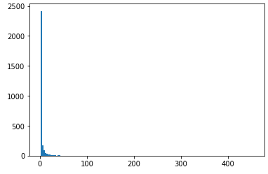
# 단어 분포 시각화
plt.hist(list(word_count_dict.values()), bins=150);
tf_idf_vect[0]를 통해 볼 수 있는 것은(0, 2788) 0번째 데이터에 2788번째 벡터에 '0.19578974958217082' TF가 계산된 값이 들어가 있다는 말 또한 .toarray()를 찍어보면 벡터의 수는 1나 단어의 수는 2850개의 자리가 있다. 그리고 tf_idf_vect[0]에서 볼 수 있듯이 특정 인덱싱 자리에만 TF가 계산된 값이 들어가 있다. 즉 0번째 문장에서 나오는 단어들의 위치와 거기에 TF값이 들어가 있는 것
이제 단어를 매핑한 후 중요 단어들을 추출 하여 보자
# 벡터 단어 매핑
invert_index_vectorizer = {v: k for k, v in vect.vocabulary_.items()}
# 중요 단어 추출
np.argsort(tf_idf_vect[0].toarray())[0][-3:] # 첫 문장에서 탑 3개
invert_index_vectorizer
{1898: 'raining',
1366: 'light',
2387: 'strobes',
2763: 'wet',
1001: 'glass',
1978: 'rhythmic',
1673: 'pace',
....} -> 단어별로 벡터번호를 받아서 표현이 되어 있다
# 중요 단어 추출
np.argsort(tf_idf_vect[0].toarray())[0][-3:] # 첫 문장에서 탑 3개
array([1984, 2387, 1978], dtype=int64)
np.argsort(tf_idf_vect.toarray())[:,-3:]
array([[1984, 2387, 1978],
[1297, 1971, 1097],
[1693, 2221, 968],
[ 690, 299, 1482],
[2823, 1951, 1454],
...)
이제 기존 데이터 프레임에 붙여서 단어로 다시 반환
# DF에 다시 단어로 붙여서 반환
top_3_word = np.argsort(tf_idf_vect.toarray())[:,-3:]
df['important_word_indexes'] = pd.Series(top_3_word.tolist())
df.head()
text → preprocessed_text로 전처리 → 워드 투 벡터 → TF처리 → TF값이 가장 높은 3개를 가져옴
이제 여기서 탑3 벡터를 워드로 변환
# 탑3 벡터를 워드로 변환
def convert_to_word(x):
word_list = []
for word in x:
word_list.append(invert_index_vectorizer[word]) #인덱스에 해당하는 키값을 찾아줌
return word_list
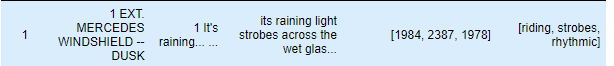
df['important_words'] = df['important_word_indexes'].apply(lambda x:convert_to_word(x))
제대로된 의미있는 단어 분석인지 봐야 한다. 3 가지의 단어를 보면 이 문장의 중심이 되고 3단어로도 이 문장의 느낌이 보이는것을 볼 수 있다. 잘 분석이 되었다.