머신러닝 06 - sklearn 알아 보기 (비지도 학습)

패스트캠퍼스 '직장인을 위한 파이썬 데이터분석 올인원 패키치 Online' 참조

 

 

 

 

01 비지도 학습이란?

• 기계 학습의 일종으로 데이터가 어떻게 구성되었는지를 알아내는 문제의 범주에 속한다. 이 방법은 지도학습 혹은 강화학습과 달리 입력값에 대한 목표치가 주어지지 않는다
• 방법으로는 차원축소, 군집화가 있다

 

 

 

02 차원축소

• feature의 개수를 줄이는 것을 넘어 특징을 추출하는 역할
• PCA, LDA, SVD 로 나뉨
• 계산 비용을 절감하고 전반적인 데이터에 대한 이해도를 높이는 효과

 

▶ PCA

• 주성분 분석(PCA)는 선형 차원 축소 기법이다. 매우 인기 있게 사용되는 차원 축소 기법 중 하나.
• 주요 특징중 하나는 분산(variance)을 최대한 보존 한다는 점
• 참조 블로그 (https://excelsior-cjh.tistory.com/167)

x,y 축으로 보는게 아닌 분산을 중점으로 P1,P2를 그려 두 선을 기점으로 특징을 추출

• 세팅시에 n_components에 1 > 면 분산을 기준으로 차원 축소, 1 < 면 해당 값을 기준으로 feature를 축소함

* 데이터 세팅

from sklearn.preprocessing import StandardScaler
from sklearn.decomposition import PCA
from sklearn import datasets
import pandas as pd

 

iris = datasets.load_iris()

 

data = iris['data']

 

df = pd.DataFrame(data, columns=iris['feature_names'])

 

df['target'] = iris['target']

pca = PCA(n_components=2)

# PCA전에 스탠다드스캐일러로 스캐일을 평균 0, 표준편차를1로 만들어야함
data_scaled = StandardScaler().fit_transform(df.loc[:, 'sepal length (cm)':'petal width (cm)'])

pca_data = pca.fit_transform(data_scaled)

pca_data[:5] #차원을 2개로 축소했기때문에 한 값에 2값만 나옴
array([[-2.26470281,  0.4800266 ],
       [-2.08096115, -0.67413356],
       [-2.36422905, -0.34190802],
       [-2.29938422, -0.59739451],
       [-2.38984217,  0.64683538]])

• 시각화로 확인

import matplotlib.pyplot as plt
from matplotlib import cm
import seaborn as sns

%matplotlib inline

plt.scatter(pca_data[:, 0], pca_data[:, 1], c=df['target']) [행 인덱스, 열 인덱스]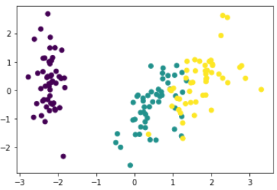

 

• 1보다 낮게하여 분산 기준으로 축소

# components > 1 하여 분산 기준으로 축소
pca = PCA(n_components=0.99)

pca_data = pca.fit_transform(data_scaled)

pca_data[:5] # 분산기준으로하면 컬럼이 몇개나올지는 랜덤임
array([[-2.26470281,  0.4800266 , -0.12770602],
       [-2.08096115, -0.67413356, -0.23460885],
       [-2.36422905, -0.34190802,  0.04420148],
       [-2.29938422, -0.59739451,  0.09129011],
       [-2.38984217,  0.64683538,  0.0157382 ]])

• 3D로 확인

from mpl_toolkits.mplot3d import Axes3D
import numpy as np 

fig = plt.figure(figsize=(10, 5))
ax = fig.add_subplot(111, projection='3d') # Axe3D object

sample_size = 50
ax.scatter(pca_data[:, 0], pca_data[:, 1], pca_data[:, 2], alpha=0.6, c=df['target'])
plt.savefig('./tmp.svg')
plt.title("ax.plot")
plt.show()

 

 

▶ LDA

• 'Linear Discriminant Analysis'로 선형 판별 분석법으로 불린다
• PCA와 비슷함. 클래스 분리를 최대화 하는 축을 찾기 위해 클래스 간 분산과 내부 분산의 비율을 최대화 하는 방식으로 차원을 축소함
• PCA는 분산을 최대한 유지하는 반면, LDA는 각각의 고유 레이블이나 클래스간의 분리를 최대한 하기위해 노력함

# LDA
from sklearn.discriminant_analysis import LinearDiscriminantAnalysis
from sklearn.preprocessing import StandardScaler

lda = LinearDiscriminantAnalysis(n_components = 2)

#스탠다드스캐일러로 스캐일을 평균 0, 표준편차를1로 만들어야함
data_scaled = StandardScaler().fit_transform(df.loc[:, 'sepal length (cm)':'petal width (cm)'])


lda_data = lda.fit_transform(data_scaled, df['target'])

lda_data[:5]
array([[ 8.06179978,  0.30042062],
       [ 7.12868772, -0.78666043],
       [ 7.48982797, -0.26538449],
       [ 6.81320057, -0.67063107],
       [ 8.13230933,  0.51446253]])

• 시각화

plt.scatter(lda_data[:, 0], lda_data[:, 1], c=df['target'])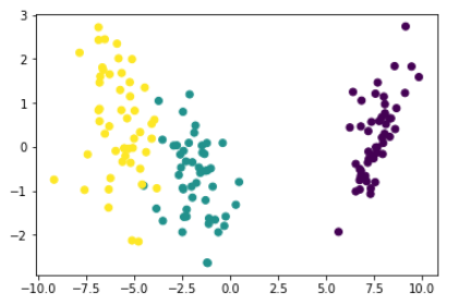

LDA VS PCA

 

 

▶ SVD

• 'Singular Value Decomposition' 으로 상품의 추천 시스템에도 활용되어지는 알고리즘 (추천시스템)
• 특이값 분해 기법. PCA와 유사한 차원 축소 기법. scikit-learn 패키지에서는 'truncated SVD (aka LSA)'를 사용함

from sklearn.decomposition import TruncatedSVD

# 스탠다드스캐일러로 스캐일을 평균 0, 표준편차를1로 만들어야함
data_scaled = StandardScaler().fit_transform(df.loc[:, 'sepal length (cm)':'petal width (cm)'])

svd = TruncatedSVD(n_components=2)

svd_data = svd.fit_transform(data_scaled, df['target'])

plt.scatter(svd_data[:, 0], svd_data[:, 1], c=df['target'])

 

 

 

 

 

 

03 군집화

• 클러스터링으로 불리며 X값을 주면 스스로 분류를 하게 된다. 
• K-Means/DBSCAN 으로 나뉜다

 

▶ K-Means

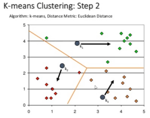
• 중심 데이터를 찾은 후 점을 찍고 거기서 가까운 점을 찾고 거기서 다시 중간 점을 찾고 계속해서 중간 점을 찾아가면서 값을 분류 함
• 주로 스팸 문자 분류, 뉴스 기사 분류등에 쓰인다.
• 하이퍼파라미터 중 'max_iter'를 조절하여 군집 분포를 조절 할 수 있다.

# K-Means
from sklearn.cluster import KMeans

#몇개의 그룹인지 모를때는 군집수를 여러번 돌려봐야함
kmeans = KMeans(n_clusters=3)

cluster_data = kmeans.fit_transform(df.loc[:, 'sepal length (cm)':'petal width (cm)'])

cluster_data[:5]
array([[3.41925061, 0.14135063, 5.0595416 ],
       [3.39857426, 0.44763825, 5.11494335],
       [3.56935666, 0.4171091 , 5.27935534],
       [3.42240962, 0.52533799, 5.15358977],
       [3.46726403, 0.18862662, 5.10433388]])
       
kmeans.labels_
array([1, 1, 1, 1, 1, 1, 1, 1, 1, 1, 1, 1, 1, 1, 1, 1, 1, 1, 1, 1, 1, 1,
       1, 1, 1, 1, 1, 1, 1, 1, 1, 1, 1, 1, 1, 1, 1, 1, 1, 1, 1, 1, 1, 1,
       1, 1, 1, 1, 1, 1, 0, 0, 2, 0, 0, 0, 0, 0, 0, 0, 0, 0, 0, 0, 0, 0,
       0, 0, 0, 0, 0, 0, 0, 0, 0, 0, 0, 2, 0, 0, 0, 0, 0, 0, 0, 0, 0, 0,
       0, 0, 0, 0, 0, 0, 0, 0, 0, 0, 0, 0, 2, 0, 2, 2, 2, 2, 0, 2, 2, 2,
       2, 2, 2, 0, 0, 2, 2, 2, 2, 0, 2, 0, 2, 0, 2, 2, 0, 0, 2, 2, 2, 2,
       2, 0, 2, 2, 2, 2, 0, 2, 2, 2, 0, 2, 2, 2, 0, 2, 2, 0])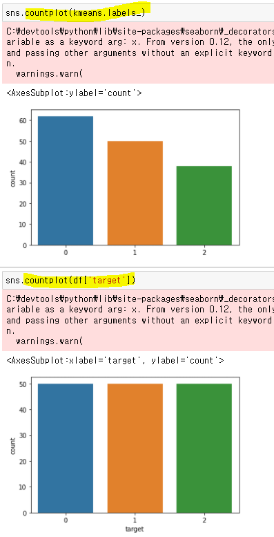

 

 

▶ DBSCAN (Density-based spatial clustering of applications with noise)

• 밀도가 높은 부분을 클러스터링 하는 방식
• 어느점을 기준으로 반경 x내에 점이 n개 이상 있으면 하나의 군집으로 인식하는 방식
• DBSCAN은 n_cluster 지정 필요 없음
• 기하학적인 clustering도 잘 찾아냄

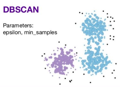
from sklearn.cluster import DBSCAN

# DBSCAN의 파라미터
# eps - 샘플간의 최대 거리
# min_sample = 몇개 이상을 그룹으로 간주 시킴
dbscan = DBSCAN(eps=0.6, min_samples=2)

# DBSCAN은 예측을 바로 시킴
dbscan_data = dbscan.fit_predict(df.loc[:, 'sepal length (cm)':'petal width (cm)'])

# 알아서 분류를 시킴
dbscan_data
array([ 0,  0,  0,  0,  0,  0,  0,  0,  0,  0,  0,  0,  0,  0,  0,  0,  0,
        0,  0,  0,  0,  0,  0,  0,  0,  0,  0,  0,  0,  0,  0,  0,  0,  0,
        0,  0,  0,  0,  0,  0,  0, -1,  0,  0,  0,  0,  0,  0,  0,  0,  1,
        1,  1,  1,  1,  1,  1,  2,  1,  1,  2,  1,  1,  1,  1,  1,  1,  1,
        1,  1,  1,  1,  1,  1,  1,  1,  1,  1,  1,  1,  1,  1,  1,  1,  1,
        1,  1,  1,  1,  1,  1,  1,  1,  2,  1,  1,  1,  1,  2,  1,  1,  1,
        1,  1,  1,  1, -1,  1,  1, -1,  1,  1,  1,  1,  1,  1,  1,  3,  1,
        1,  1,  1,  1,  1,  1,  1,  1,  1,  1,  1,  1,  3,  1,  1,  1,  1,
        1,  1,  1,  1,  1,  1,  1,  1,  1,  1,  1,  1,  1,  1],
      dtype=int64)

 

 

04 군집화 평가 - 실루엣 스코어

• 클러스터링의 품질을 정량적으로 평가해주는 지표
• 1 - 품질이 좋음
  0 - 품질이 않좋음 (클러스터링의 의미가 없음)
  음수 - 잘못 분류됨

from sklearn.metrics import silhouette_samples, silhouette_score

score = silhouette_score(data_scaled, kmeans.labels_)

score
0.44366157397640527

samples = silhouette_samples(data_scaled, kmeans.labels_)

samples[:5]
array([0.73318987, 0.57783809, 0.68201014, 0.62802187, 0.72693222])

• 시각화

def plot_silhouette(X, num_cluesters):
    for n_clusters in num_cluesters:
        # Create a subplot with 1 row and 2 columns
        fig, (ax1, ax2) = plt.subplots(1, 2)
        fig.set_size_inches(18, 7)

        # The 1st subplot is the silhouette plot
        # The silhouette coefficient can range from -1, 1 but in this example all
        # lie within [-0.1, 1]
        ax1.set_xlim([-0.1, 1])
        # The (n_clusters+1)*10 is for inserting blank space between silhouette
        # plots of individual clusters, to demarcate them clearly.
        ax1.set_ylim([0, len(X) + (n_clusters + 1) * 10])
    
        # Initialize the clusterer with n_clusters value and a random generator
        # seed of 10 for reproducibility.
        clusterer = KMeans(n_clusters=n_clusters, random_state=10)
        cluster_labels = clusterer.fit_predict(X)
    
        # The silhouette_score gives the average value for all the samples.
        # This gives a perspective into the density and separation of the formed
        # clusters
        silhouette_avg = silhouette_score(X, cluster_labels)
        print("For n_clusters =", n_clusters,
              "The average silhouette_score is :", silhouette_avg)
    
        # Compute the silhouette scores for each sample
        sample_silhouette_values = silhouette_samples(X, cluster_labels)
    
        y_lower = 10
        for i in range(n_clusters):
            # Aggregate the silhouette scores for samples belonging to
            # cluster i, and sort them
            ith_cluster_silhouette_values = \
                sample_silhouette_values[cluster_labels == i]
    
            ith_cluster_silhouette_values.sort()
    
            size_cluster_i = ith_cluster_silhouette_values.shape[0]
            y_upper = y_lower + size_cluster_i
    
            color = cm.nipy_spectral(float(i) / n_clusters)
            ax1.fill_betweenx(np.arange(y_lower, y_upper),
                              0, ith_cluster_silhouette_values,
                              facecolor=color, edgecolor=color, alpha=0.7)
    
            # Label the silhouette plots with their cluster numbers at the middle
            ax1.text(-0.05, y_lower + 0.5 * size_cluster_i, str(i))
    
            # Compute the new y_lower for next plot
            y_lower = y_upper + 10  # 10 for the 0 samples
    
        ax1.set_title("The silhouette plot for the various clusters.")
        ax1.set_xlabel("The silhouette coefficient values")
        ax1.set_ylabel("Cluster label")
    
        # The vertical line for average silhouette score of all the values
        ax1.axvline(x=silhouette_avg, color="red", linestyle="--")
    
        ax1.set_yticks([])  # Clear the yaxis labels / ticks
        ax1.set_xticks([-0.1, 0, 0.2, 0.4, 0.6, 0.8, 1])
    
        # 2nd Plot showing the actual clusters formed
        colors = cm.nipy_spectral(cluster_labels.astype(float) / n_clusters)
        ax2.scatter(X[:, 0], X[:, 1], marker='.', s=30, lw=0, alpha=0.7,
                    c=colors, edgecolor='k')
    
        # Labeling the clusters
        centers = clusterer.cluster_centers_
        # Draw white circles at cluster centers
        ax2.scatter(centers[:, 0], centers[:, 1], marker='o',
                    c="white", alpha=1, s=200, edgecolor='k')
    
        for i, c in enumerate(centers):
            ax2.scatter(c[0], c[1], marker='$%d$' % i, alpha=1,
                        s=50, edgecolor='k')
    
        ax2.set_title("The visualization of the clustered data.")
        ax2.set_xlabel("Feature space for the 1st feature")
        ax2.set_ylabel("Feature space for the 2nd feature")
    
        plt.suptitle(("Silhouette analysis for KMeans clustering on sample data "
                      "with n_clusters = %d" % n_clusters),
                     fontsize=14, fontweight='bold')
    
        plt.show()

plot_silhouette(data_scaled, [2,3,4,5])

• 스캐일화가 된 데이터와 클러스터링 개수를 리스트 형태로 넣으면 된다

빨간 점선은 평균 실루엣 계수를 의미하고 빨간점이 넘어갔으면 좋은 평가.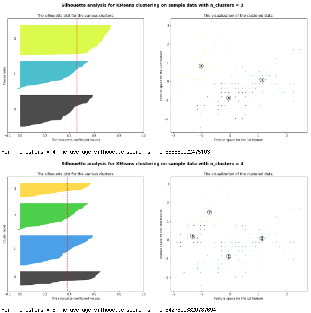 

• 비교를 해보면 2개의 군집을 놓을때가 평균이 제일 높게 나온다. 즉 성능이 제일 좋다는 말