머신러닝 05 - sklearn 알아 보기 (앙상블)
패스트캠퍼스 '직장인을 위한 파이썬 데이터분석 올인원 패키치 Online' 참조
01 앙상블 이란?
- 여러개의 머신러닝 모델을 이용해 최적의 답을 찾아내는 기법
- 여러 모델을 이용하여 데이터를 학습하고 그 이후 모든 모델의 예측결과를 평균하여 예측함
- 앙상블 대표 기법은 다음과 같다
보팅(Voting) - 투표를 통해 결과 도출
배깅(Bagging) - 샘플 중복 생성을 통해 결과 도출
부스팅(Boosting) - 이전 오차를 보완하면서 가중치 부여
스태킹(Stacking) - 여러 모델을 기반으로 예측된 결과를 통해 meta 모델이 다시 한번 예측
02 앙상블 진행을 위한 세팅
- 필요 데이터 세팅
import pandas as pd
import numpy as np
from IPython.display import Image

np.set_printoptions(suppress=True)

from sklearn.datasets import load_boston

data = load_boston()

df = pd.DataFrame(data['data'], columns=data['feature_names'])

df['MEDV'] = data['target']

df.head()

# 데이터셋 분리
from sklearn.model_selection import train_test_split
x_train, x_test, y_train, y_test = train_test_split(df.drop('MEDV', 1), df['MEDV'])

# 평가지표
from sklearn.metrics import mean_absolute_error, mean_squared_error
* 모델별 성능 확인을 위한 함수
import matplotlib.pyplot as plt
import seaborn as sns
my_predictions = {}
colors = ['r', 'c', 'm', 'y', 'k', 'khaki', 'teal', 'orchid', 'sandybrown',
'greenyellow', 'dodgerblue', 'deepskyblue', 'rosybrown', 'firebrick',
'deeppink', 'crimson', 'salmon', 'darkred', 'olivedrab', 'olive',
'forestgreen', 'royalblue', 'indigo', 'navy', 'mediumpurple', 'chocolate',
'gold', 'darkorange', 'seagreen', 'turquoise', 'steelblue', 'slategray',
'peru', 'midnightblue', 'slateblue', 'dimgray', 'cadetblue', 'tomato'
]
def plot_predictions(name_, pred, actual):
df = pd.DataFrame({'prediction': pred, 'actual': y_test})
df = df.sort_values(by='actual').reset_index(drop=True)
plt.figure(figsize=(12, 9))
plt.scatter(df.index, df['prediction'], marker='x', color='r')
plt.scatter(df.index, df['actual'], alpha=0.7, marker='o', color='black')
plt.title(name_, fontsize=15)
plt.legend(['prediction', 'actual'], fontsize=12)
plt.show()
def mse_eval(name_, pred, actual):
global predictions
global colors
plot_predictions(name_, pred, actual)
mse = mean_squared_error(pred, actual)
my_predictions[name_] = mse
y_value = sorted(my_predictions.items(), key=lambda x: x[1], reverse=True)
df = pd.DataFrame(y_value, columns=['model', 'mse'])
print(df)
min_ = df['mse'].min() - 10
max_ = df['mse'].max() + 10
length = len(df)
plt.figure(figsize=(10, length))
ax = plt.subplot()
ax.set_yticks(np.arange(len(df)))
ax.set_yticklabels(df['model'], fontsize=15)
bars = ax.barh(np.arange(len(df)), df['mse'])
for i, v in enumerate(df['mse']):
idx = np.random.choice(len(colors))
bars[i].set_color(colors[idx])
ax.text(v + 2, i, str(round(v, 3)), color='k', fontsize=15, fontweight='bold')
plt.title('MSE Error', fontsize=18)
plt.xlim(min_, max_)
plt.show()
def remove_model(name_):
global my_predictions
try:
del my_predictions[name_]
except KeyError:
return False
return True
def plot_coef(columns, coef):
coef_df = pd.DataFrame(list(zip(columns, coef)))
coef_df.columns=['feature', 'coef']
coef_df = coef_df.sort_values('coef', ascending=False).reset_index(drop=True)
fig, ax = plt.subplots(figsize=(9, 7))
ax.barh(np.arange(len(coef_df)), coef_df['coef'])
idx = np.arange(len(coef_df))
ax.set_yticks(idx)
ax.set_yticklabels(coef_df['feature'])
fig.tight_layout()
plt.show()
* 필요 라이브러리 세팅
# 평가지표
from sklearn.metrics import mean_absolute_error, mean_squared_error
from sklearn.linear_model import LinearRegression
from sklearn.linear_model import Ridge
from sklearn.linear_model import Lasso
from sklearn.linear_model import ElasticNet
from sklearn.preprocessing import StandardScaler, MinMaxScaler, RobustScaler
from sklearn.pipeline import make_pipeline
from sklearn.preprocessing import PolynomialFeatures

linear_reg = LinearRegression(n_jobs=-1)
linear_reg.fit(x_train, y_train)
pred = linear_reg.predict(x_test)
mse_eval('LinearRegression', pred, y_test)

ridge = Ridge()
ridge.fit(x_train, y_train)
pred = ridge.predict(x_test)
mse_eval('Ridge(alpha=1)', pred, y_test)

lasso = Lasso()
lasso.fit(x_train, y_train)
pred = lasso.predict(x_test)
mse_eval('Lasso(alpha=0.01)', pred, y_test)

elasticnet = ElasticNet()
elasticnet.fit(x_train, y_train)
pred = elasticnet.predict(x_test)
mse_eval('ElasticNet(l1_ratio=0.8)', pred, y_test)

elasticnet_pipeline = make_pipeline(
    PolynomialFeatures(degree=2, include_bias=False),
    StandardScaler(),
    ElasticNet(alpha=0.1, l1_ratio=0.2)
)
elasticnet_pred = elasticnet_pipeline.fit(x_train, y_train).predict(x_test)
mse_eval('Standard ElasticNet', elasticnet_pred, y_test)

poly_pipeline = make_pipeline(
    PolynomialFeatures(degree=2, include_bias=False),
    StandardScaler(),
    ElasticNet(alpha=0.1, l1_ratio=0.2)
)
poly_pred = poly_pipeline.fit(x_train, y_train).predict(x_test)
mse_eval('Poly ElasticNet', poly_pred, y_test)
03 보팅 회귀
- 단어 뜻 그대로 투표를 통해 결정하는 방식. 배깅과 투표라는 점에서 비슷하나 2가지의 차이가 있음
1. Voting은 다른 알고리즘 모델을 조합하여 사용
2. Bagging은 같은 알고리즘내에서 다른 샘플 조합을 사용
from sklearn.ensemble import VotingRegressor

# 보팅을 위한 모델들 세팅
# 반드시 Tuple 형태로 정의
single_models = [
    ('linear_reg', linear_reg),
    ('ridge', ridge),
    ('lasso', lasso),
    ('elasticnet_pipeline', elasticnet_pipeline),
    ('poly_pipeline', poly_pipeline)
]

# 보팅 세팅
voting_regressor = VotingRegressor(single_models, n_jobs=-1)

voting_pred = voting_regressor.predict(x_test)

mse_eval('Voting Ensemble', voting_pred, y_test)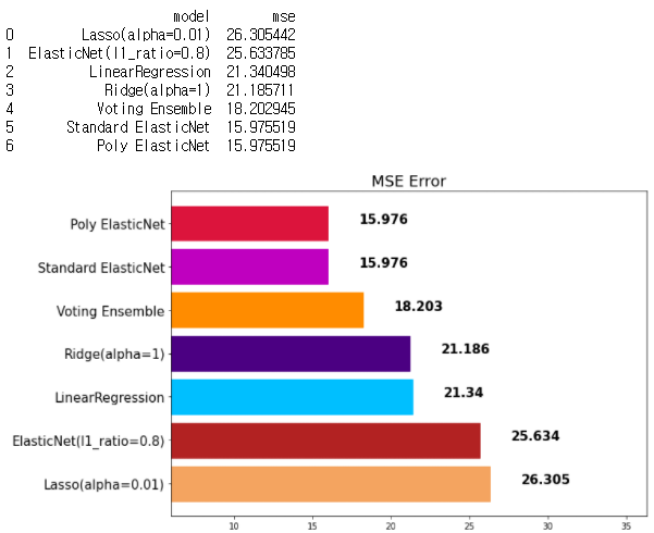
▶ 보팅 분류
- 분류는 0,1로 예측을 하는 이진 분류로 보팅 방식에서 'soft'/'hard'로 나뉜다.
- 하드 방식은 가장 많이 나온 값을 바로 채택하게되고, 소프트는 모든 클래스들의 평균을 구하여 가장 높은값으로 채택함
- 주로 소프트를 많이 씀
분류기 모델을 만들때, Voting 앙상블은 1가지의 중요한 parameter가 있습니다.

# 보팅 분류
from sklearn.ensemble import VotingClassifier

voting = {'hard', 'soft'}

hard로 설정한 경우

class를 0, 1로 분류 예측을 하는 이진 분류를 예로 들어 보겠습니다.

Hard Voting 방식에서는 결과 값에 대한 다수 class를 차용합니다.

classification을 예로 들어 보자면, 분류를 예측한 값이 1, 0, 0, 1, 1 이었다고 가정한다면 1이 3표, 0이 2표를 받았기 때문에 Hard Voting 방식에서는 1이 최종 값으로 예측을 하게 됩니다.

soft

soft vote 방식은 각각의 확률의 평균 값을 계산한다음에 가장 확률이 높은 값으로 확정짓게 됩니다.

가령 class 0이 나올 확률이 (0.4, 0.9, 0.9, 0.4, 0.4)이었고, class 1이 나올 확률이 (0.6, 0.1, 0.1, 0.6, 0.6) 이었다면,

class 0이 나올 최종 확률은 (0.4+0.9+0.9+0.4+0.4) / 5 = 0.44,
class 1이 나올 최종 확률은 (0.6+0.1+0.1+0.6+0.6) / 5 = 0.4
가 되기 때문에 앞선 Hard Vote의 결과와는 다른 결과 값이 최종 으로 선출되게 됩니다.
04 배깅
- 'Bootstrap Aggregating'의 줄임말
- Bootstrop = Sample + Aggregating 으로 여러개의 데이터셋 중첩을 허용하고 거기서 샘플링하여 분할하는 방식
- 예로 데이터 셋의 구성이 [1,2,3,4,5] 라면 A=[1,2,3], B=[1,3,4], C=[2,3,5]

- Voting은 여러 알고리즘 조합, Bagging은 하나의 단일 알고리즘에 대하여 여러 샘플을 조합
- 대표적인 'Bagging' 앙상블로는 배깅과 랜덤포레스트가 있고 랜덤포레스트를 더 많이 씀
▶ 랜덤 포레스트
- Decision Tree기반 배깅 앙상블
- 앙상블 중 굉장히 인기가 많은 모델. 사용이 쉽고 성능도 우수함
from sklearn.ensemble import RandomForestRegressor, RandomForestClassifier

rtr = RandomForestRegressor()
rtr.fit(x_train, y_train)

rtr_pred = rtr.predict(x_test)
mse_eval('RandomForest Ensemble', rtr_pred, y_test)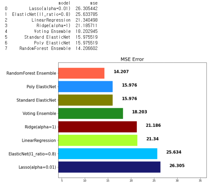
- 앞으로 단일 모델보다는 앙상블을 많이 쓰게 된다. 이때 주요 하이퍼파라미터는 다음과 같다
random_state: 랜덤 시드 고정 값. 고정해두고 튜닝할 것! n_jobs: CPU 사용 갯수 max_depth: 깊어질 수 있는 최대 깊이. 과대적합 방지용 n_estimators: 앙상블하는 트리의 갯수 max_features: 최대로 사용할 feature의 갯수. 과대적합 방지용 min_samples_split: 트리가 분할할 때 최소 샘플의 갯수. default=2. 과대적합 방지용
05 부스팅
- 약한 학습기를 순차적으로 학습을 하되, 이전 학습에 대하여 잘못 예측된 데이터에 가중치를 부여해 오차를 보완해나가는 방식
- 성능은 매우 우수하나 약점을 보완하려고 하기때문에 잘못된 레이블링이나 아웃라이어에 필요 이상으로 민감하고 학습 시간이 오래 걸린다는 단점이 있다
- 대표적인 부스팅 앙상블은 아래와 같다
- AdaBoost
- GradientBoost
- LightGBM (LGBM)
- XGBoost
▶ GradientBoost - 성능이 우수하나 학습시간이 해도해도 너무 느림
gbr = GradientBoostingRegressor(random_state=42)
gbr.fit(x_train, y_train)
gbr_pred = gbr.predict(x_test)
mse_eval('GradientBoost Ensemble', gbr_pred, y_test)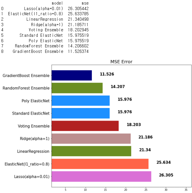
주요 Hyperparameter
- random_state: 랜덤 시드 고정 값. 고정해두고 튜닝할 것!
- n_jobs: CPU 사용 갯수
- learning_rate: 학습율. 너무 큰 학습율은 성능을 떨어뜨리고, 너무 작은 학습율은 학습이 느리다. 적절한 값을 찾아야함. n_estimators와 같이 튜닝. default=0.1
- n_estimators: 부스팅 스테이지 수. (랜덤포레스트 트리의 갯수 설정과 비슷한 개념). default=100
- subsample: 샘플 사용 비율 (max_features와 비슷한 개념). 과대적합 방지용
- min_samples_split: 노드 분할시 최소 샘플의 갯수. default=2. 과대적합 방지용
▶ XGBoost
- scikit-learn 패키지가 아닙니다.
- 성능이 우수함
- GBM보다는 빠르고 성능도 향상되었습니다.
- 여전히 학습시간이 매우 느리다
pip install xgboost
* VS Code나 아나콘다에 설치를 해줘야 사용 가능
#XGBoost
from xgboost import XGBRegressor, XGBClassifier
xgb = XGBRegressor(random_state=42)
xgb.fit(x_train, y_train)
xgb_pred = xgb.predict(x_test)
mse_eval('XGBoost', xgb_pred, y_test)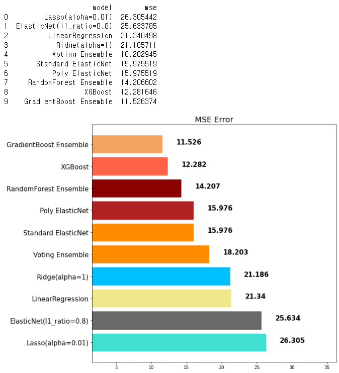
06 LigthGBM
- scikit-learn 패키지가 아님
- 성능이 좋고 XGBoost보다 속도가 뛰어남
pip install lightgbm
* VS CODE나 아나콘다에 설치 필요
# LigthGBM
from lightgbm import LGBMRegressor, LGBMClassifier
lgbm = LGBMRegressor(random_state=42)
lgbm.fit(x_train, y_train)
lgbm_pred = lgbm.predict(x_test)
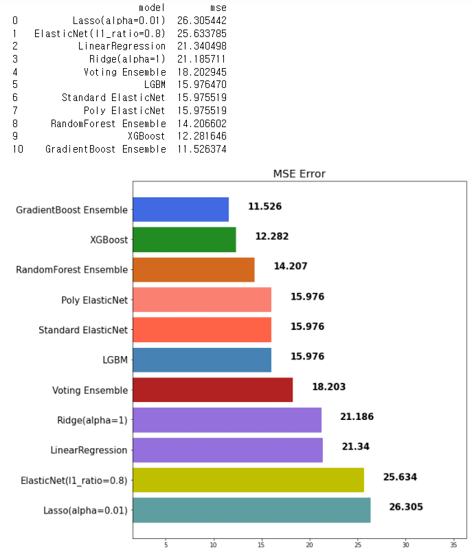
mse_eval('LGBM', lgbm_pred, y_test)* max_features와 비슷한 개념의 파라미터가 존재
- colsample_bytree: 샘플 사용 비율 (max_features와 비슷한 개념). 과대적합 방지용. default=1.0)
07 스태킹
- 개별 모델이 예측한 데이터를 기반으로 final_estimator를 종합하여 예측 수행
- 성능을 극으로 끌어올릴 때 활용, 과대적합을 유발 할 수 있음(특히 데이터셋이 적은 경우)
# 스태킹
from sklearn.ensemble import StackingRegressor

stack_models = [
    ('elasticnet', poly_pipeline),
    ('randomforest', rtr),
    ('gbr', gbr),
    ('lgbm', lgbm)
]

stack_reg = StackingRegressor(stack_models, final_estimator=xgb, n_jobs=-1)

stack_reg.fit(x_train, y_train)
stack_pred = stack_reg.predict(x_test)
mse_eval('Stacking Ensemble', stack_pred, y_test)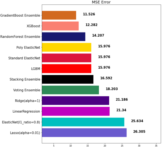
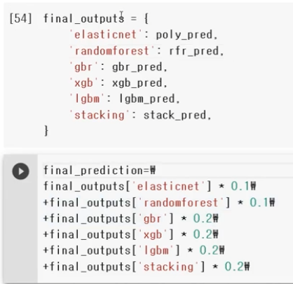
08 Weighted Belnding
- 각 모델의 예측값에 대하여 weight를 계산하고 그 값을 곱하여 최종 결과 계산
- 가중치를 조절하여 최종 결과가 나오는데 가중치의 합은 1.0이 되도록 해야함
09 앙상블 모델 총평
- 앙상블은 실무에서 많이 쓰임
- 대체적으로 단일 모델 대비 성능이 매우 좋음
- 앙상블을 다시 한번 앙상블하는 기법인 스태킹과 웨이트블렌딩을 참고해도 좋음
- 앙상블 모델은 적절한 하이퍼파라미터 튜닝이 필요함
- 앙상블 모델은 대체적으로 학습 시간이 더 오래 걸림, 즉 모델 튜닝에도 오래 걸림
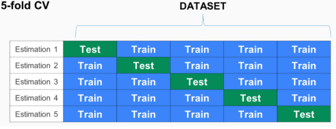
▶ Cross Validation (CV로 부름)
- 모델을 평가하는 하나의 방법. K-겹 교차검증을 많이 활용함
- K-겹 교차 검증 - 모든 데이터가 최소 한 번은 테스트셋으로 쓰이도록 하는 것
- [예시]
- Estimation 1일때,
- Estimation 2일때,
from sklearn.model_selection import KFold

n_splits = 5
kfold = KFold(n_splits=n_splits, random_state=42, shuffle=True)

X = np.array(df.drop('MEDV', 1))
Y = np.array(df['MEDV'])

# 속도가 빠른 LGBM 을 사용하고 이 모델 테스트
lgbm_fold = LGBMRegressor(random_state=42)

i = 1
total_error = 0
for train_index, test_index in kfold.split(X): # 'kfold.split' 이 알아서 교차 검증 데이터를 나눔
    x_train_fold, x_test_fold = X[train_index], X[test_index]
    y_train_fold, y_test_fold = Y[train_index], Y[test_index]
    lgbm_pred_fold = lgbm_fold.fit(x_train_fold, y_train_fold).predict(x_test_fold)
    error = mean_squared_error(lgbm_pred_fold, y_test_fold)
    print('Fold = {}, prediction score = {:.2f}'.format(i, error))
    total_error += error
    i+=1
print('---'*10)
print('Average Error: %s' % (total_error / n_splits))

Fold = 1, prediction score = 8.34
Fold = 2, prediction score = 10.40
Fold = 3, prediction score = 17.58
Fold = 4, prediction score = 6.94
Fold = 5, prediction score = 12.16
------------------------------
Average Error: 11.083201392666322
▶ 하이퍼 파라미터 튜닝
- 지금까지 보면 각각의 모델들은 자기만의 하이퍼파라미터를 튜닝 할 수 있다. 하지만 이 튜닝시에 경우의 수가 너무 많기 떄문에 적절하게 자동으로 찾아줄 수 있는 도움이 필요
- 하지만 '반드시 손 튜닝에 익숙해 진 후에 자동화로 넘어가야함'
- sklearn에서 자주 사용되는 하이퍼파라미터 튜닝을 돕는 클래스는 2가지.
1. RandomizedSearchCV
2. GridSearchCV - 적용 방법
1. 사용할 Search 방법을 선택
2. hyperparameter 도메인을 설정 (max_depth, n_estimators..등등)
3. 학습을 시킨 후, 기다림
4. 도출된 결과 값을 모델에 적용하고 성능을 비교
- RandomizedSearchCV
- 모든 매개 변수 값이 시도되는 것이 아니라 지정된 분포에서 고정 된 수의 매개 변수 설정이 샘플링됨
- 시도 된 매개 변수 설정의 수는 n_iter에 의해 제공
주요 Hyperparameter (LGBM)
- random_state: 랜덤 시드 고정 값. 고정해두고 튜닝할 것!
- n_jobs: CPU 사용 갯수
- learning_rate: 학습율. 너무 큰 학습율은 성능을 떨어뜨리고, 너무 작은 학습율은 학습이 느리다. 적절한 값을 찾아야함. n_estimators와 같이 튜닝. default=0.1
- n_estimators: 부스팅 스테이지 수. (랜덤포레스트 트리의 갯수 설정과 비슷한 개념). default=100
- max_depth: 트리의 깊이. 과대적합 방지용. default=3.
- colsample_bytree: 샘플 사용 비율 (max_features와 비슷한 개념). 과대적합 방지용. default=1.0
- n_iter 값을 조절하여, 총 몇 회의 시도를 진행할 것인지 정의합니다.
(회수가 늘어나면, 더 좋은 parameter를 찾을 확률은 올라가지만, 그만큼 시간이 오래걸립니다.)
params = {
    'n_estimators':[200,500,1000,2000],
    'learning_rate':[0.1, 0.05, 0.01],
    'max_depth':[6,7,8],
    'colsample_bytree':[0.8,0.9,0.1],
    'subsample':[0.8,0.9,1.0]
}

from sklearn.model_selection import RandomizedSearchCV

# cv = 교차검증 겹 설정
# n_iter = 랜덤값 25회 시도
# scoring = 설정된 에러 값을 구함
clf = RandomizedSearchCV(LGBMRegressor(), params, random_state=42, cv=3, n_iter=25, scoring='neg_mean_squared_error')

clf.fit(x_train, y_train)
clf.best_score_
-11.559039903559041
clf.best_params_
{'subsample': 1.0,
'n_estimators': 1000,
'max_depth': 7,
'learning_rate': 0.05,
'colsample_bytree': 0.9}
* 나온값들로 돌려봄
lgbm_best = LGBMRegressor(n_estimators=1000, subsample=1.0, max_depth=7, learning_rate=0.05,colsample_bytree=0.9 )
lgbm_best_pred = lgbm_best.fit(x_train, y_train).predict(x_test)
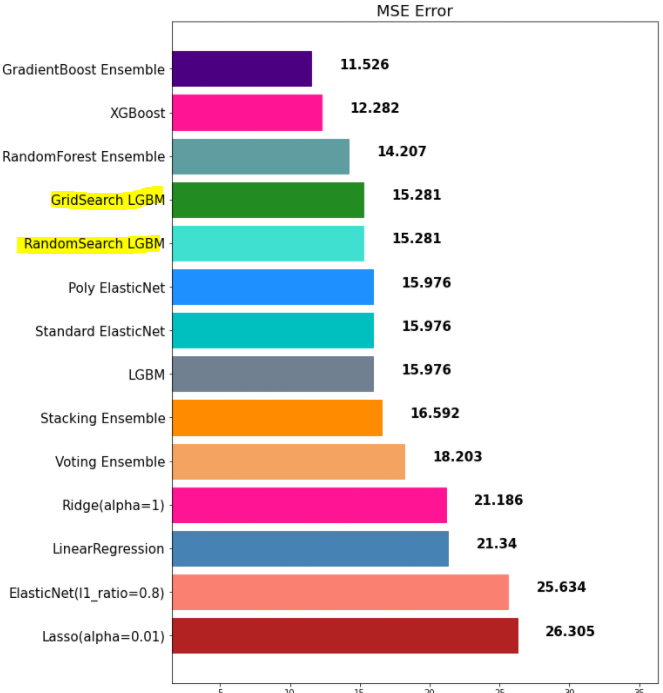
mse_eval('RandomSearch LGBM', lgbm_best_pred, y_test)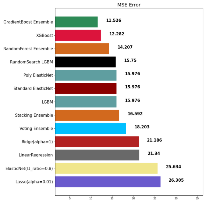
- GridSearchCV
- 모든 매개 변수 값에 대하여 '완전 탐색'을 함
- 최적화할 파라미터가 많으면 시간이 매우 오래 걸림
* 손 튜닝을 먼저해서 최적의 파람 구간을 찾자!

params = {
    'n_estimators': [500, 1000],
    'learning_rate': [0.1, 0.05, 0.01],
    'max_depth': [7, 8],
    'colsample_bytree': [0.8, 0.9],
    'subsample': [0.8, 0.9,],
}

from sklearn.model_selection import GridSearchCV

grid_search = GridSearchCV(LGBMRegressor(), params, cv=3, n_jobs=-1, scoring='neg_mean_squared_error')

grid_search.fit(x_train, y_train)

grid_search.best_params_
{'colsample_bytree': 0.9,
 'learning_rate': 0.05,
 'max_depth': 8,
 'n_estimators': 1000,
 'subsample': 0.8}
lgbm_best = LGBMRegressor(n_estimators=1000, subsample=0.8, max_depth=8, learning_rate=0.05,colsample_bytree=0.9)
lgbm_best_pred = lgbm_best.fit(x_train, y_train).predict(x_test)
mse_eval('RandomSearch LGBM', lgbm_best_pred, y_test)